


vectorbt学习_41DMA之一基础策略
773 字
4 分钟
vectorbt学习_41DMA之一基础策略
基于vectorbt的基础双均线策略
01,基础配置信息
#conda envs:vectorbt_envimport warningsimport vectorbt as vbtimport numpy as npimport pandas as pdfrom datetime import datetime, timedeltaimport pytzfrom dateutil.parser import parseimport ipywidgets as widgetsfrom copy import deepcopyfrom tqdm import tqdmimport imageiofrom IPython import displayimport plotly.graph_objects as goimport itertoolsimport dateparserimport gcimport mathfrom tools import dbtools
warnings.filterwarnings("ignore")
pd.set_option('display.max_rows',500)pd.set_option('display.max_columns',500)pd.set_option('display.width',1000)02,行情获取和可视化
a,时间交易参数配置
# Enter your parameters hereseed = 42symbol = '002594.XSHE'metric = 'total_return'
start_date = datetime(2020, 1, 1, tzinfo=pytz.utc) # time period for analysis, must be timezone-awareend_date = datetime(2023,1,1, tzinfo=pytz.utc)time_buffer = timedelta(days=100) # buffer before to pre-calculate SMA/EMA, best to set to max windowfreq = '1D'
vbt.settings.portfolio['init_cash'] = 10000. # 100$vbt.settings.portfolio['fees'] = 0.0025 # 0.25%vbt.settings.portfolio['slippage'] = 0.0025 # 0.25%b,获取行情和行情mask
# Download data with time buffercols = ['Open', 'High', 'Low', 'Close', 'Volume']# ohlcv_wbuf = vbt.YFData.download(symbol, start=start_date-time_buffer, end=end_date).get(cols)
ohlcv_wbuf=dbtools.MySQLData.download(symbol).get() # 自带工具类查询assert(~ohlcv_wbuf.empty)ohlcv_wbuf = ohlcv_wbuf.astype(np.float64)
print("origin ohlcv_wbuf size:",ohlcv_wbuf.shape)print(ohlcv_wbuf.columns)
# Create a copy of data without time bufferwobuf_mask = (ohlcv_wbuf.index >= start_date) & (ohlcv_wbuf.index <= end_date) # mask without buffer
ohlcv = ohlcv_wbuf.loc[wobuf_mask, :]
print("wobuf_mask ohlcv size:",ohlcv.shape)
# Plot the OHLC dataohlcv.vbt.ohlcv.plot().show_svg() # 绘制蜡烛图# remove show_svg() to display interactive chart!origin ohlcv_wbuf size: (978, 5)Index(['Open', 'High', 'Low', 'Close', 'Volume'], dtype='object')wobuf_mask ohlcv size: (728, 5)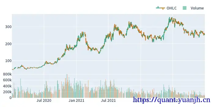
03,指标计算和可视化
# fig.show_svg()fast_window = 35slow_window = 60
# Pre-calculate running windows on data with time bufferfast_ma = vbt.MA.run(ohlcv_wbuf['Close'], fast_window)slow_ma = vbt.MA.run(ohlcv_wbuf['Close'], slow_window)
print(fast_ma.ma.shape)print(slow_ma.ma.shape)
# Remove time bufferfast_ma = fast_ma[wobuf_mask]slow_ma = slow_ma[wobuf_mask]
# there should be no nans after removing time bufferassert(~fast_ma.ma.isnull().any())assert(~slow_ma.ma.isnull().any())
print(fast_ma.ma.shape)print(slow_ma.ma.shape)
fig = ohlcv['Open'].vbt.plot(trace_kwargs=dict(name='Price'))fig = fast_ma.ma.vbt.plot(trace_kwargs=dict(name='Fast MA'), fig=fig)fig = slow_ma.ma.vbt.plot(trace_kwargs=dict(name='Slow MA'), fig=fig)fig.show_svg()(978,)(978,)(728,)(728,)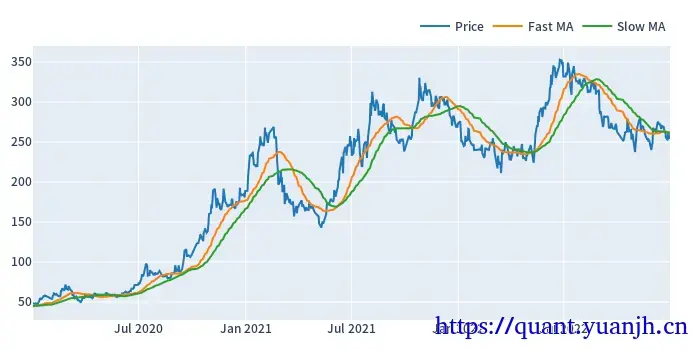
04,信号计算,可视化
# 信号计算dmac_entries = fast_ma.ma_crossed_above(slow_ma)dmac_exits = fast_ma.ma_crossed_below(slow_ma)
# 行情-指标-信号可视化fig = ohlcv['Close'].vbt.plot(trace_kwargs=dict(name='Price'))fig = fast_ma.ma.vbt.plot(trace_kwargs=dict(name='Fast MA'), fig=fig)fig = slow_ma.ma.vbt.plot(trace_kwargs=dict(name='Slow MA'), fig=fig)fig = dmac_entries.vbt.signals.plot_as_entry_markers(ohlcv['Close'], fig=fig)fig = dmac_exits.vbt.signals.plot_as_exit_markers(ohlcv['Close'], fig=fig)fig.show_svg()
# (单独)信号可视化fig = dmac_entries.vbt.signals.plot(trace_kwargs=dict(name='Entries'))dmac_exits.vbt.signals.plot(trace_kwargs=dict(name='Exits'), fig=fig).show_svg()
# 信号的统计信息dmac_entries.vbt.signals.stats(settings=dict(other=dmac_exits))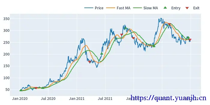
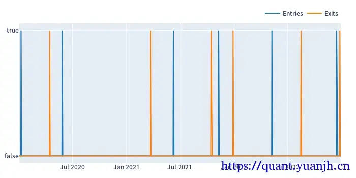
Start 2020-01-02 00:00:00+00:00End 2022-12-30 00:00:00+00:00Period 728Total 6Rate [%] 0.824176Total Overlapping 0Overlapping Rate [%] 0.0First Index 2020-01-08 00:00:00+00:00Last Index 2022-12-16 00:00:00+00:00Norm Avg Index [-1, 1] -0.002751Distance -> Other: Min 7.0Distance -> Other: Max 200.0Distance -> Other: Mean 76.333333Distance -> Other: Std 66.503133Total Partitions 6Partition Rate [%] 100.0Partition Length: Min 1.0Partition Length: Max 1.0Partition Length: Mean 1.0Partition Length: Std 0.0Partition Distance: Min 90.0Partition Distance: Max 252.0Partition Distance: Mean 142.6Partition Distance: Std 65.305436dtype: object05,交易统计
a,基准比对
dmac_pf = vbt.Portfolio.from_signals(ohlcv['Close'], dmac_entries, dmac_exits)# Print statsprint(dmac_pf.stats())
# Now build portfolio for a "Hold" strategy# Here we buy once at the beginning and sell at the endhold_entries = pd.Series.vbt.signals.empty_like(dmac_entries)hold_entries.iloc[0] = Truehold_exits = pd.Series.vbt.signals.empty_like(hold_entries)hold_exits.iloc[-1] = Truehold_pf = vbt.Portfolio.from_signals(ohlcv['Close'], hold_entries, hold_exits)
# Equityfig = dmac_pf.value().vbt.plot(trace_kwargs=dict(name='Value (DMAC)'))hold_pf.value().vbt.plot(trace_kwargs=dict(name='Value (Hold)'), fig=fig).show_svg()Start 2020-01-02 00:00:00+00:00End 2022-12-30 00:00:00+00:00Period 728Start Value 10000.0End Value 56343.449364Total Return [%] 463.434494Benchmark Return [%] 433.464812Max Gross Exposure [%] 100.0Total Fees Paid 1154.406013Max Drawdown [%] 37.462162Max Drawdown Duration 319.0Total Trades 6Total Closed Trades 6Total Open Trades 0Open Trade PnL 0.0Win Rate [%] 66.666667Best Trade [%] 192.432267Worst Trade [%] -14.196623Avg Winning Trade [%] 72.994385Avg Losing Trade [%] -9.136247Avg Winning Trade Duration 104.0Avg Losing Trade Duration 21.0Profit Factor 5.95588Expectancy 7723.908227dtype: object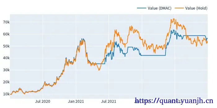
b,交易详情和可视化
# Plot tradesprint(dmac_pf.trades.records.head(5))dmac_pf.trades.plot().show_svg() id col size entry_idx entry_price entry_fees exit_idx exit_price exit_fees pnl return direction status parent_id0 0 0 210.452345 4 47.398200 24.937656 66 57.775200 30.397316 2128.529014 0.213385 0 1 01 1 0 210.612793 94 57.443250 30.245708 294 168.547575 88.745689 23281.000774 1.924323 0 1 12 2 0 174.421504 346 202.505000 88.303067 430 282.621675 123.238244 13762.529659 0.389639 0 1 23 3 0 157.697151 448 311.035650 122.623590 483 268.327500 105.786206 -6963.363374 -0.141966 0 1 34 4 0 179.995892 566 233.913325 105.258594 636 327.110175 147.196219 16522.595293 0.392429 0 1 4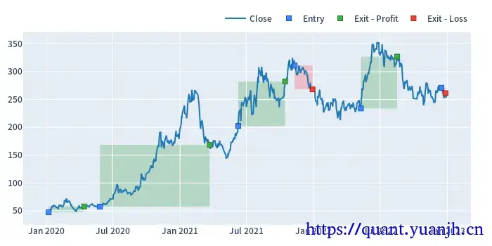
文章分享
如果这篇文章对你有帮助,欢迎分享给更多人!
vectorbt学习_41DMA之一基础策略
https://quant.yuanjh.cn/posts/f6621c56/ 相关文章 智能推荐
1
vectorbt学习_60DC之一基础策略
06重拾量化 / btvt 2024-12-10
2
vectorbt学习_10PortfolioOptimization
06重拾量化 / btvt 2023-11-05
3
vectorbt学习_08PortingBTStrategy
06重拾量化 / btvt 2023-10-28
4
vectorbt学习_09WalkForwardOptimization
06重拾量化 / btvt 2023-10-28
5
vectorbt学习_06MACDVolume
06重拾量化 / btvt 2023-10-22
随机文章 随机推荐
欢迎来到我的博客!这是一则示例公告。
音乐
暂未播放
0:00 0:00
55
8
10
107,410
0 天
0 天前