


2433 字
12 分钟
vectorbt学习_10PortfolioOptimization
投资组合优化,需要一定背景知识,否则不清楚整篇文章干嘛的,达到什么目的。
“马科维茨”投资组合模型实践——第三章 投资组合优化:最小方差与最大夏普比率:https://www.jianshu.com/p/400758e58768
随机搜索最优权重
构造随机权重
np.random.seed(42)
# Generate random weights, n timesweights = []for i in range(num_tests): w = np.random.random_sample(len(symbols)) w = w / np.sum(w) weights.append(w)
print(len(weights))2000
weights[array([0.18205878, 0.46212909, 0.35581214]), array([0.65738127, 0.17132261, 0.17129612]), array([0.03807826, 0.56784481, 0.39407693]), array([0.41686469, 0.01211874, 0.57101657]), array([0.67865488, 0.173111 , 0.14823412]), array([0.18115758, 0.3005149 , 0.51832752]),
3列是由于本例子使用的symbols标的有3个symbols = [ '510050.XSHG', '510300.XSHG', '159901.XSHE']数据准备
# Build column hierarchy such that one weight corresponds to one price series# 3列数据,变为3*num_tests=》3*2000=6000列_price = price.vbt.tile(num_tests, keys=pd.Index(np.arange(num_tests), name='symbol_group'))_price = _price.vbt.stack_index(pd.Index(np.concatenate(weights), name='weights'))
print(_price.columns)MultiIndex([( 0.18205877561639985, 0, '510050.XSHG'), ( 0.46212908544657766, 0, '510300.XSHG'), ,,, ( 0.34668046300795724, 1999, '510300.XSHG'), ( 0.1067148038247113, 1999, '159901.XSHE')], names=['weights', 'symbol_group', 'symbol'], length=6000)tile用法样例
price.vbt.tile(3, keys=pd.Index(list('abc'), name='symbol_group'))#简单来说,原始数据列,复制出3份,3份在column的mulitindex索引标识为a,b,c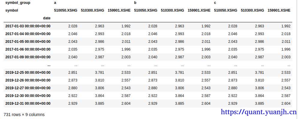
stack_index用法样例
num_tests= 3tmpp=price.vbt.tile(num_tests, keys=pd.Index(np.arange(num_tests), name='symbol_group'))weights = []for i in range(3): w = np.random.random_sample(len(symbols)) w = w / np.sum(w) weights.append(w)print(np.concatenate(weights))# [0.28035754 0.08989454 0.62974792 0.41627195 0.11541703 0.46831101 0.02859779 0.75619858 0.21520363]tmpp.vbt.stack_index(pd.Index(np.concatenate(weights), name='weights'))# 将新增的pd.Index,attach到原有的multiIndex上。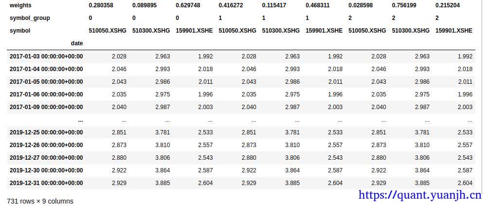
生成订单
# Run simulationpf = vbt.Portfolio.from_orders( close=_price, size=size,# size只有 初始的第一行,意味着不会调仓 size_type='targetpercent', # size中保存的数据是标的百分比,由于单组weight已经做了sum=1的计算保证 # 购买时,是OrderContext.cash_now的百分比。 # 卖出时,是OrderContext.position_now的百分比。 # 卖空时为OrderContext.free_cash_now的百分比。 # 卖出和卖空(即反转仓位)时,是OrderContext.position_now和OrderContext.free_cash_now的百分比。
group_by='symbol_group',# 结果分组 cash_sharing=True) # all weights sum to 1, no shorting, and 100% investment in risky assets
print(len(pf.orders))6000波动率收益回报率,可视化
annualized_return = pf.annualized_return()# 前文截图case为例:# a 2.273208# b -0.737391# Name: annualized_return, dtype: float64
annualized_return.index = pf.annualized_volatility()# 前文截图case为例:# a 0.090345# b 0.091265# Name: annualized_volatility, dtype: float64
# 可见是2个series
# 此时annualized_return是一个series,index=波动率,value=收益率annualized_return.vbt.scatterplot( trace_kwargs=dict( mode='markers', marker=dict( color=pf.sharpe_ratio(), colorbar=dict( title='sharpe_ratio' ), size=5, opacity=0.7 ) ), xaxis_title='annualized_volatility', yaxis_title='annualized_return').show_svg()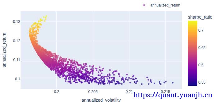
取得最优组合信息
# Get index of the best group according to the target metricbest_symbol_group = pf.sharpe_ratio().idxmax()
print(best_symbol_group)400
print(pf.sharpe_ratio().max())print(pf.sharpe_ratio().idxmax())print(pf.sharpe_ratio()[pf.sharpe_ratio().idxmax()])0.72779659957785614000.7277965995778561
# Print best weightsprint(weights[best_symbol_group])[0.94197268 0.03054375 0.02748357]
# Compute default statsprint(pf.iloc[best_symbol_group].stats())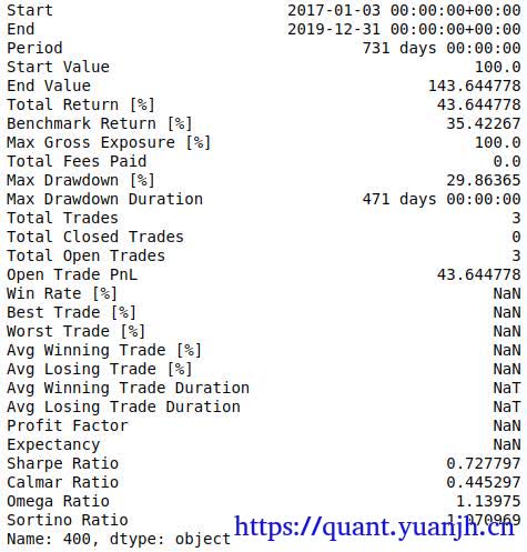
月再平衡(重置回初始权重)
收益计算
按照月重新平衡,虽然再平衡权重没变,但由于标的价格变化,购买时的size对应的targetpercent,其实是现金比例,所以实际仓位也会变化。等于在原始持续持有的基础上,卖出了上涨幅度大的(由于上涨,导致reset时,实际targetpercent高于初始取值,所以会卖出部分,维持资金占比)。
# Select the first index of each monthrb_mask = ~_price.index.to_period('m').duplicated()
print(rb_mask.sum())36 # 说明共36个月这部分如何理解?
_price.index.to_period('m')# =># PeriodIndex(['2017-01', '2017-01', '2017-01', '2017-01', '2017-01', '2017-01', '2017-01', '2017-01', '2017-01', '2017-01', ... '2019-12', '2019-12', '2019-12', '2019-12', '2019-12', '2019-12', '2019-12', '2019-12', '2019-12', '2019-12'], dtype='period[M]', name='date', length=731)
_price.index.to_period('m').duplicated()# array([False, True, True, True, True, True, True, True, True, True, True, True, True, True, True, True, True, True, False, True, True, True, True, True, True, True, True, True, True, True, True, True, True, True, True, True, False, True, True, True, True, True, True, True, True, True, True, True, True, True, True, True, True, True, True, True, True, True, True, False, True, True, True, True, True, True, True, True, True, True, True, True, 731个,false的都是每个月的第一日
~_price.index.to_period('m').duplicated()# 取反后,每个月第一日从False变为True再平衡日,重新设置权重
rb_size = np.full_like(_price, np.nan)rb_size[rb_mask, :] = np.concatenate(weights) # allocate at mask # 再平衡日,重设权重
print(rb_size.shape)(731, 6000)重新计算再平衡收益
# Run simulation, with rebalancing monthlyrb_pf = vbt.Portfolio.from_orders( close=_price, size=rb_size, size_type='targetpercent', group_by='symbol_group', cash_sharing=True, call_seq='auto' # important: sell before buy)
print(len(rb_pf.orders))rb_best_symbol_group = rb_pf.sharpe_ratio().idxmax()
print(rb_best_symbol_group)print(weights[rb_best_symbol_group])
216000400[0.94197268 0.03054375 0.02748357]
print(rb_pf.iloc[rb_best_symbol_group].stats())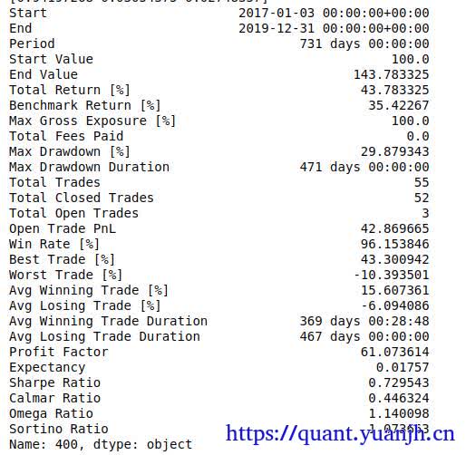
权值可视化
def plot_allocation(rb_pf): # Plot weights development of the portfolio rb_asset_value = rb_pf.asset_value(group_by=False) rb_value = rb_pf.value() rb_idxs = np.flatnonzero((rb_pf.asset_flow() != 0).any(axis=1)) rb_dates = rb_pf.wrapper.index[rb_idxs] fig = (rb_asset_value.vbt / rb_value).vbt.plot( trace_names=symbols, trace_kwargs=dict( stackgroup='one' ) ) for rb_date in rb_dates: fig.add_shape( dict( xref='x', yref='paper', x0=rb_date, x1=rb_date, y0=0, y1=1, line_color=fig.layout.template.layout.plot_bgcolor ) ) fig.show_svg()plot_allocation(rb_pf.iloc[rb_best_symbol_group]) # best group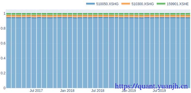
搜索和30日再平衡
srb_sharpe = np.full(price.shape[0], np.nan)
@njitdef pre_sim_func_nb(c, every_nth): # Define rebalancing days c.segment_mask[:, :] = False c.segment_mask[every_nth::every_nth, :] = True return ()
@njitdef find_weights_nb(c, price, num_tests): # Find optimal weights based on best Sharpe ratio returns = (price[1:] - price[:-1]) / price[:-1] returns = returns[1:, :] # cannot compute np.cov with NaN mean = nanmean_nb(returns) cov = np.cov(returns, rowvar=False) # masked arrays not supported by Numba (yet) best_sharpe_ratio = -np.inf weights = np.full(c.group_len, np.nan, dtype=np.float_)
for i in range(num_tests): # Generate weights w = np.random.random_sample(c.group_len) w = w / np.sum(w)
# Compute annualized mean, covariance, and Sharpe ratio p_return = np.sum(mean * w) * ann_factor p_std = np.sqrt(np.dot(w.T, np.dot(cov, w))) * np.sqrt(ann_factor) sharpe_ratio = p_return / p_std if sharpe_ratio > best_sharpe_ratio: best_sharpe_ratio = sharpe_ratio weights = w
return best_sharpe_ratio, weights
@njitdef pre_segment_func_nb(c, find_weights_nb, history_len, ann_factor, num_tests, srb_sharpe): if history_len == -1: # Look back at the entire time period close = c.close[:c.i, c.from_col:c.to_col] else: # Look back at a fixed time period if c.i - history_len <= 0: return (np.full(c.group_len, np.nan),) # insufficient data close = c.close[c.i - history_len:c.i, c.from_col:c.to_col]
# Find optimal weights best_sharpe_ratio, weights = find_weights_nb(c, close, num_tests) srb_sharpe[c.i] = best_sharpe_ratio
# Update valuation price and reorder orders size_type = SizeType.TargetPercent direction = Direction.LongOnly order_value_out = np.empty(c.group_len, dtype=np.float_) for k in range(c.group_len): col = c.from_col + k c.last_val_price[col] = c.close[c.i, col] sort_call_seq_nb(c, weights, size_type, direction, order_value_out)
return (weights,)
@njitdef order_func_nb(c, weights): col_i = c.call_seq_now[c.call_idx] return order_nb( weights[col_i], c.close[c.i, c.col], size_type=SizeType.TargetPercent )
ann_factor = returns.vbt.returns.ann_factor
# Run simulation using a custom order functionsrb_pf = vbt.Portfolio.from_order_func( price, order_func_nb, pre_sim_func_nb=pre_sim_func_nb, pre_sim_args=(30,), pre_segment_func_nb=pre_segment_func_nb, pre_segment_args=(find_weights_nb, -1, ann_factor, num_tests, srb_sharpe), cash_sharing=True, group_by=True)
# Plot best Sharpe ratio at each rebalancing daypd.Series(srb_sharpe, index=price.index).vbt.scatterplot(trace_kwargs=dict(mode='markers')).show_svg()
print(srb_pf.stats())from_order_func(有点复杂,暂跳过)
先搞清楚from_order_func,参考:https://vectorbt.dev/api/portfolio/base/#vectorbt.portfolio.base.Portfolio.from_order_func
# Run simulation using a custom order functionsrb_pf = vbt.Portfolio.from_order_func( price, #行情信息 order_func_nb,#订单生成函数 pre_sim_func_nb=pre_sim_func_nb,# Function called before simulation. Defaults to no_pre_func_nb(). pre_sim_args=(30,),# Packed arguments passed to pre_sim_func_nb. Defaults to (). pre_segment_func_nb=pre_segment_func_nb,# Function called before each segment. Defaults to no_pre_func_nb(). pre_segment_args=(find_weights_nb, -1, ann_factor, num_tests, srb_sharpe), #Packed arguments passed to pre_segment_func_nb. Defaults to (). cash_sharing=True, # Whether to share cash within the same group. # If group_by is None, group_by becomes True to form a single group with cash sharing. group_by=True)关于from_order_func,几个比较容易混淆的重要的函数
order_func_nb: callable 订单生成功能。post_order_func_nb: callable 订单处理后调用的回调。
pre(post)_sim_func_nb: callable 模拟之前调用的函数。默认为no_pre_func_nb()。
pre/post_group_func_nb: 在每组之前调用的函数。默认为no_pre_func_nb()。 仅当 为 False 时才调用row_wise。
pre/post_row_func_nb: callable 在每行之前调用的函数。默认为no_pre_func_nb()。 仅当为 True 时才调用row_wise。
pre/post_segment_func_nb: callable # 段是组和行之间的交集。它是一个实体,定义如何以及以何种顺序处理同一组和行中的元素。 在每个段之前调用的函数。默认为no_pre_func_nb()。 segment_mask: int或array_like的bool 是否应执行特定段的掩码。 提供一个整数将激活每第 n 行。提供布尔值或布尔值数组将广播到行数和组数。 不与close和一起广播broadcast_named_args,仅针对最终形状。 call_pre_segment: bool 是否打电话pre_segment_func_nb不管segment_mask。 call_post_segment: bool 是否打电话post_segment_func_nb不管segment_mask。执行官方提供最简单demo
import numpy as npimport pandas as pdfrom datetime import datetimefrom numba import njit
import vectorbt as vbtfrom vectorbt.utils.colors import adjust_opacityfrom vectorbt.utils.enum_ import map_enum_fieldsfrom vectorbt.base.reshape_fns import broadcast, flex_select_auto_nb, to_2d_arrayfrom vectorbt.portfolio.enums import SizeType, Direction, NoOrder, OrderStatus, OrderSidefrom vectorbt.portfolio import nb
@njitdef order_func_nb(c, size): return nb.order_nb(size=size)
close = pd.Series([1, 2, 3, 4, 5])pf = vbt.Portfolio.from_order_func(close, order_func_nb, 10)
nb.order_nb(size=5) #本身返回一个order对象,故order_func_nb可看做order构造函数,生成一系列orderOrder(size=5.0, price=inf, size_type=0, direction=2, fees=0.0, fixed_fees=0.0, slippage=0.0, min_size=0.0, max_size=inf, size_granularity=nan, reject_prob=0.0, lock_cash=False, allow_partial=True, raise_reject=False, log=False)
print(pf.assets())print(pf.cash())
0 10.01 20.02 30.03 40.04 40.0dtype: float640 90.01 70.02 40.03 0.04 0.0dtype: float64
输出分析:每次买入10份,每份价格分别:1,2,3,4,5,交易记录和消耗资金如下buy:10*1(-10)buy:10*2(-20)buy:10*3(-30)buy:10*4(-40)assets对应股票份额,每天增加10,最多买到40就到头了(资金不足)有效边界法(PyPortfolioOpt)
# Calculate expected returns and sample covariance amtrixavg_returns = expected_returns.mean_historical_return(price)symbol510050.XSHG 0.135305510300.XSHG 0.098036159901.XSHE 0.096895dtype: float64
cov_mat = risk_models.sample_cov(price) # 协方差矩阵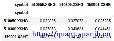
# Get weights maximizing the Sharpe ratioef = EfficientFrontier(avg_returns, cov_mat)weights = ef.max_sharpe()weightsOrderedDict([('510050.XSHG', 1.0), ('510300.XSHG', 0.0), ('159901.XSHE', 0.0)])
clean_weights = ef.clean_weights()clean_weightsOrderedDict([('510050.XSHG', 1.0), ('510300.XSHG', 0.0), ('159901.XSHE', 0.0)])
pyopt_weights = np.array([clean_weights[symbol] for symbol in symbols])print(pyopt_weights)[1. 0. 0.]填充初始权值
pyopt_size = np.full_like(price, np.nan)pyopt_size[0, :] = pyopt_weights # allocate at first timestamp, do nothing afterwards
print(pyopt_size[:5])print(pyopt_size.shape)[[ 1. 0. 0.] [nan nan nan] [nan nan nan] [nan nan nan] [nan nan nan]](731, 3)只进行一次初始化时的交易回测
# Run simulation with weights from PyPortfolioOptpyopt_pf = vbt.Portfolio.from_orders( close=price, size=pyopt_size, size_type='targetpercent', group_by=True, cash_sharing=True)
print(len(pyopt_pf.orders))1
收益统计print(pyopt_pf.stats())Start 2017-01-03 00:00:00+00:00End 2019-12-31 00:00:00+00:00Period 731 days 00:00:00Start Value 100.0End Value 144.428008Total Return [%] 44.428008Benchmark Return [%] 35.42267Max Gross Exposure [%] 100.0Total Fees Paid 0.0Max Drawdown [%] 29.64467Max Drawdown Duration 462 days 00:00:00Total Trades 1Total Closed Trades 0Total Open Trades 1Open Trade PnL 44.428008Win Rate [%] NaNBest Trade [%] NaNWorst Trade [%] NaNAvg Winning Trade [%] NaNAvg Losing Trade [%] NaNAvg Winning Trade Duration NaTAvg Losing Trade Duration NaTProfit Factor NaNExpectancy NaNSharpe Ratio 0.735009Calmar Ratio 0.455758Omega Ratio 1.14102Sortino Ratio 1.082667Name: group, dtype: object有效边界的按月再平衡
原文中有这么一段描述
You can't use third-party optimization packages within Numba (yet). #不确定为啥Here you have two choices:1) Use os.environ['NUMBA_DISABLE_JIT'] = '1' before all imports to disable Numba completely 2) Disable Numba for the function, but also for every other function in the stack that calls itWe will demonstrate the second option.重写了weight方法
def pyopt_find_weights(sc, price, num_tests): # no @njit decorator = it's a pure Python function # Calculate expected returns and sample covariance matrix price = pd.DataFrame(price, columns=symbols) avg_returns = expected_returns.mean_historical_return(price) cov_mat = risk_models.sample_cov(price)
# Get weights maximizing the Sharpe ratio ef = EfficientFrontier(avg_returns, cov_mat) weights = ef.max_sharpe() clean_weights = ef.clean_weights() weights = np.array([clean_weights[symbol] for symbol in symbols]) best_sharpe_ratio = base_optimizer.portfolio_performance(weights, avg_returns, cov_mat)[2]
return best_sharpe_ratio, weights计算组合收益
pyopt_srb_sharpe = np.full(price.shape[0], np.nan)
# Run simulation with a custom order functionpyopt_srb_pf = vbt.Portfolio.from_order_func( price, order_func_nb, pre_sim_func_nb=pre_sim_func_nb, pre_sim_args=(30,), pre_segment_func_nb=pre_segment_func_nb.py_func, # run pre_segment_func_nb as pure Python function pre_segment_args=(pyopt_find_weights, -1, ann_factor, num_tests, pyopt_srb_sharpe), cash_sharing=True, group_by=True, use_numba=False # run simulate_nb as pure Python function)夏普值的可视化
pd.Series(pyopt_srb_sharpe, index=price.index).vbt.scatterplot(trace_kwargs=dict(mode='markers')).show_svg()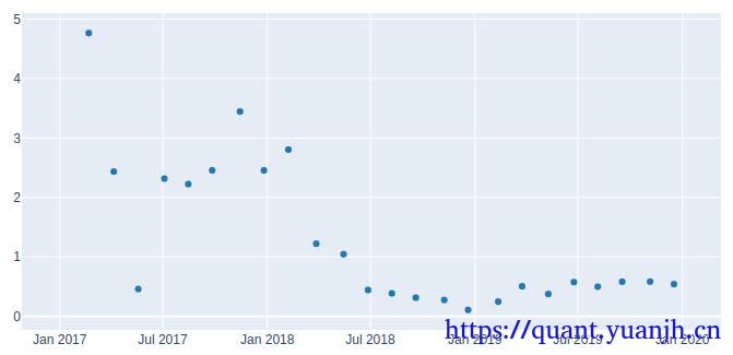
绩效评估
print(pyopt_srb_pf.stats())Start 2017-01-03 00:00:00+00:00End 2019-12-31 00:00:00+00:00Period 731 days 00:00:00Start Value 100.0End Value 130.474091Total Return [%] 30.474091Benchmark Return [%] 35.42267Max Gross Exposure [%] 100.0Total Fees Paid 0.0Max Drawdown [%] 31.0145Max Drawdown Duration 471 days 00:00:00Total Trades 13Total Closed Trades 12Total Open Trades 1Open Trade PnL 26.174785Win Rate [%] 58.333333Best Trade [%] 23.399167Worst Trade [%] -11.947833Avg Winning Trade [%] 8.563981Avg Losing Trade [%] -4.049498Avg Winning Trade Duration 107 days 03:25:42.857142856Avg Losing Trade Duration 78 days 00:00:00Profit Factor 1.788768Expectancy 0.358275Sharpe Ratio 0.563374Calmar Ratio 0.309651Omega Ratio 1.108617Sortino Ratio 0.820358Name: group, dtype: object权值可视化
plot_allocation(pyopt_srb_pf)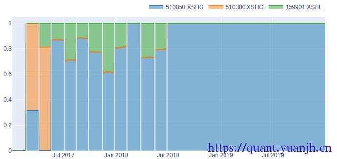
附录
Portfolio.from_orders
参考:https://vectorbt.dev/api/portfolio/base/#from-orders
样例
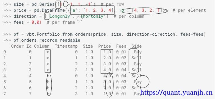
需要注意的是size<1>,-1,1,-1需要结合不同direction会生成不同的sell,buy信号,shortonly时的size=1表示卖出。
from_signals
vectorbt学习_10PortfolioOptimization
/posts/quant/06c7414f/ 部分信息可能已经过时
公告
欢迎来到黄金矿工的博客!