


743 字
4 分钟
vectorbt学习_42DMA之二网格参数优选
本文在上一篇文章(vectorbt学习_16DMA之一基础策略)基础上,采用网格分析法分析策略的最优参数。
01,基础配置信息
#conda envs:vectorbt_envimport warningsimport vectorbt as vbtimport numpy as npimport pandas as pdfrom datetime import datetime, timedeltaimport pytzfrom dateutil.parser import parseimport ipywidgets as widgetsfrom copy import deepcopyfrom tqdm import tqdmimport imageiofrom IPython import displayimport plotly.graph_objects as goimport itertoolsimport dateparserimport gcimport mathfrom tools import dbtools
warnings.filterwarnings("ignore")
pd.set_option('display.max_rows',500)pd.set_option('display.max_columns',500)pd.set_option('display.width',1000)02,行情获取和可视化
a,时间交易参数配置
# Enter your parameters hereseed = 42symbol = '002594.XSHE'metric = 'total_return'
start_date = datetime(2020, 1, 1, tzinfo=pytz.utc) # time period for analysis, must be timezone-awareend_date = datetime(2023,1,1, tzinfo=pytz.utc)time_buffer = timedelta(days=100) # buffer before to pre-calculate SMA/EMA, best to set to max windowfreq = '1D'
vbt.settings.portfolio['init_cash'] = 10000. # 100$vbt.settings.portfolio['fees'] = 0.0025 # 0.25%vbt.settings.portfolio['slippage'] = 0.0025 # 0.25%b,获取行情和行情mask
# Download data with time buffercols = ['Open', 'High', 'Low', 'Close', 'Volume']# ohlcv_wbuf = vbt.YFData.download(symbol, start=start_date-time_buffer, end=end_date).get(cols)
ohlcv_wbuf=dbtools.MySQLData.download(symbol).get() # 自带工具类查询assert(~ohlcv_wbuf.empty)ohlcv_wbuf = ohlcv_wbuf.astype(np.float64)
print("origin ohlcv_wbuf size:",ohlcv_wbuf.shape)print(ohlcv_wbuf.columns)
# Create a copy of data without time bufferwobuf_mask = (ohlcv_wbuf.index >= start_date) & (ohlcv_wbuf.index <= end_date) # mask without buffer
ohlcv = ohlcv_wbuf.loc[wobuf_mask, :]
print("wobuf_mask ohlcv size:",ohlcv.shape)
# Plot the OHLC dataohlcv.vbt.ohlcv.plot().show_svg() # 绘制蜡烛图# remove show_svg() to display interactive chart!origin ohlcv_wbuf size: (978, 5)Index(['Open', 'High', 'Low', 'Close', 'Volume'], dtype='object')wobuf_mask ohlcv size: (728, 5)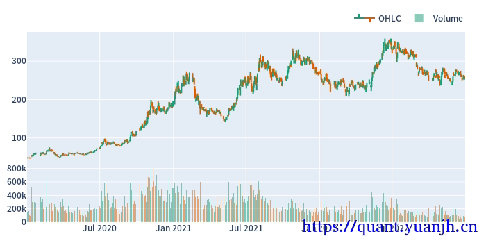
10,网格参数寻优
a,基础参数设置
min_window = 10max_window = 60
metric = 'total_return'b,多维(联合索引)指标
# Pre-calculate running windows on data with time bufferfast_ma, slow_ma = vbt.MA.run_combs( ohlcv_wbuf['Close'], np.arange(min_window, max_window+1), r=2, short_names=['fast_ma', 'slow_ma'])print("##### 111 #####")print(fast_ma.ma.shape)print(slow_ma.ma.shape)print(fast_ma.ma.columns)print(slow_ma.ma.columns)
# Remove time bufferfast_ma = fast_ma[wobuf_mask]slow_ma = slow_ma[wobuf_mask]print("##### 222 #####")print(fast_ma.ma.shape)print(slow_ma.ma.shape)fast_ma.ma.columns##### 111 #####(978, 1275)(978, 1275)Int64Index([10, 10, 10, 10, 10, 10, 10, 10, 10, 10, ... 56, 56, 56, 56, 57, 57, 57, 58, 58, 59], dtype='int64', name='fast_ma_window', length=1275)Int64Index([11, 12, 13, 14, 15, 16, 17, 18, 19, 20, ... 57, 58, 59, 60, 58, 59, 60, 59, 60, 60], dtype='int64', name='slow_ma_window', length=1275)##### 222 #####(728, 1275)(728, 1275)
Int64Index([10, 10, 10, 10, 10, 10, 10, 10, 10, 10, ... 56, 56, 56, 56, 57, 57, 57, 58, 58, 59], dtype='int64', name='fast_ma_window', length=1275)c,多维(联合索引)信号
# We perform the same steps, but now we have 4851 columns instead of 1# Each column corresponds to a pair of fast and slow windows# Generate crossover signalsdmac_entries = fast_ma.ma_crossed_above(slow_ma)dmac_exits = fast_ma.ma_crossed_below(slow_ma)print(dmac_entries.columns) # the same for dmac_exitsMultiIndex([(10, 11), (10, 12), (10, 13), (10, 14), (10, 15), (10, 16), (10, 17), (10, 18), (10, 19), (10, 20), ... (56, 57), (56, 58), (56, 59), (56, 60), (57, 58), (57, 59), (57, 60), (58, 59), (58, 60), (59, 60)], names=['fast_ma_window', 'slow_ma_window'], length=1275)d,多维(联合索引)信号回测,最佳参数组
# Build portfoliodmac_pf = vbt.Portfolio.from_signals(ohlcv['Close'], dmac_entries, dmac_exits)# Calculate performance of each window combinationdmac_perf = dmac_pf.deep_getattr(metric)
print(dmac_perf.shape)print(dmac_perf.index)
print("dmac_perf.idxmax()")print(dmac_perf.idxmax()) # your optimal window combination(1275,)MultiIndex([(10, 11), (10, 12), (10, 13), (10, 14), (10, 15), (10, 16), (10, 17), (10, 18), (10, 19), (10, 20), ... (56, 57), (56, 58), (56, 59), (56, 60), (57, 58), (57, 59), (57, 60), (58, 59), (58, 60), (59, 60)], names=['fast_ma_window', 'slow_ma_window'], length=1275)dmac_perf.idxmax()(35, 60)e,网格选优热力图
# Convert this array into a matrix of shape (99, 99): 99 fast windows x 99 slow windowsdmac_perf_matrix = dmac_perf.vbt.unstack_to_df(symmetric=True, index_levels='fast_ma_window', column_levels='slow_ma_window')print("dmac_perf_matrix.shape")print(dmac_perf_matrix.shape)
dmac_perf_matrix.vbt.heatmap( xaxis_title='Slow window', yaxis_title='Fast window').show_svg()# remove show_svg() for interactivitydmac_perf_matrix.shape(51, 51)('fast_ma_window', 'slow_ma_window') 10 11 12 13 14 15 16 17 18 19 20 21 22 23 24 25 26 27 28 29 30 31 32 33 34 35 36 37 38 39 40 41 42 43 44 45 46 47 48 49 50 51 52 53 54 55 56 57 58 59 60(fast_ma_window, slow_ma_window)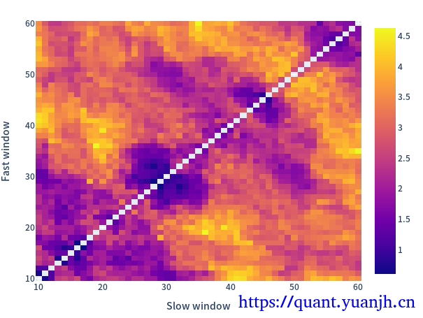
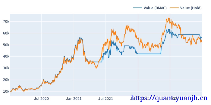
11,最佳参数回测图
部分信息可能已经过时
公告
欢迎来到黄金矿工的博客!