


对比用backtrader实现策略和vectorbt实现策略的异同
数据查询和可视化
price=dbtools.MySQLData.download('510050.XSHG',start_dt=start_date_str,end_dt=end_date_str) # 自定义工具类查询data = price.get()
ohlcv_wbuf.vbt.ohlcv.plot().show_svg()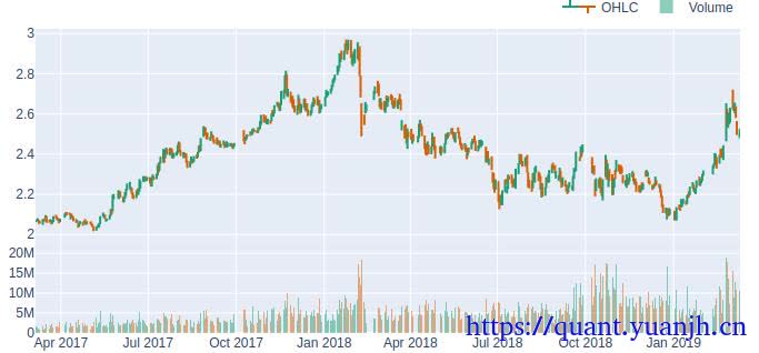
bt策略
需要对backtrader有基础的了解。
定义cerebro,broker
class FullMoney(PercentSizer): params = ( ('percents', 100 - fees), )
data_bt = bt.feeds.PandasData( dataname=ohlcv_wbuf, openinterest=-1, datetime=None, timeframe=bt.TimeFrame.Minutes, compression=1 )
cerebro = bt.Cerebro(quicknotify=True)cerebro.adddata(data_bt)broker = cerebro.getbroker()broker.set_coc(True) # cheat-on-closebroker.setcommission(commission=fees/100)#, name=coin_target)broker.setcash(init_cash)cerebro.addsizer(FullMoney)cerebro.addanalyzer(bt.analyzers.TradeAnalyzer, _name="ta")cerebro.addanalyzer(bt.analyzers.SQN, _name="sqn")cerebro.addanalyzer(bt.analyzers.Transactions, _name="transactions")定义RSI策略
class StrategyBase(bt.Strategy): def __init__(self): self.order = None self.last_operation = "SELL" self.status = "DISCONNECTED" self.buy_price_close = None self.pending_order = False self.commissions = []
def notify_data(self, data, status, *args, **kwargs): self.status = data._getstatusname(status)
def short(self): self.sell()
def long(self): self.buy_price_close = self.data0.close[0] self.buy()
def notify_order(self, order): self.pending_order = False if order.status in [order.Submitted, order.Accepted]: self.order = order return
elif order.status in [order.Completed]: self.commissions.append(order.executed.comm)
if order.isbuy(): self.last_operation = "BUY"
else: # Sell self.buy_price_close = None self.last_operation = "SELL"
self.order = None
class BasicRSI(StrategyBase): params = dict( #入参申明 period_ema_fast=fast_window, period_ema_slow=slow_window, rsi_bottom_threshold=rsi_bottom, rsi_top_threshold=rsi_top )
def __init__(self): StrategyBase.__init__(self)
self.ema_fast = bt.indicators.EMA(period=self.p.period_ema_fast) self.ema_slow = bt.indicators.EMA(period=self.p.period_ema_slow) self.rsi = bt.talib.RSI(self.data, timeperiod=14) #指标计算 #self.rsi = bt.indicators.RelativeStrengthIndex()
self.profit = 0 self.stop_loss_flag = True
def update_indicators(self): #指标更新 self.profit = 0 if self.buy_price_close and self.buy_price_close > 0: self.profit = float( self.data0.close[0] - self.buy_price_close) / self.buy_price_close
def next(self): self.update_indicators()
if self.order: # waiting for pending order return
# stop Loss ''' if self.profit < -0.03: self.short() '''
# take Profit ''' if self.profit > 0.03: self.short() '''
# reset stop loss flag if self.rsi > self.p.rsi_bottom_threshold: self.stop_loss_flag = False
if self.last_operation != "BUY": # 这里需要注意,由于rsi可能持续小于阈值,需避免持续的下单 # if self.rsi < 30 and self.ema_fast > self.ema_slow: if self.rsi < self.p.rsi_bottom_threshold: # and not self.stop_loss_flag: self.long()
if self.last_operation != "SELL": if self.rsi > self.p.rsi_top_threshold: self.short()运行策略
cerebro.addstrategy(BasicRSI)initial_value = cerebro.broker.getvalue()print('Starting Portfolio Value: %.2f' % initial_value)result = cerebro.run()
Starting Portfolio Value: 100.62 #期末终值,比最初100多了0.62打印交易摘要信息
def print_trade_analysis(analyzer): # 将analyzer的一部分信息按照特定格式打印出来 # Get the results we are interested in if not analyzer.get("total"): return
total_open = analyzer.total.open total_closed = analyzer.total.closed total_won = analyzer.won.total total_lost = analyzer.lost.total win_streak = analyzer.streak.won.longest lose_streak = analyzer.streak.lost.longest pnl_net = round(analyzer.pnl.net.total, 2) strike_rate = round((total_won / total_closed) * 2)
# Designate the rows h1 = ['Total Open', 'Total Closed', 'Total Won', 'Total Lost'] h2 = ['Strike Rate', 'Win Streak', 'Losing Streak', 'PnL Net'] r1 = [total_open, total_closed, total_won, total_lost] r2 = [strike_rate, win_streak, lose_streak, pnl_net]
# Check which set of headers is the longest. if len(h1) > len(h2): header_length = len(h1) else: header_length = len(h2)
# Print the rows print_list = [h1, r1, h2, r2] row_format = "{:<15}" * (header_length + 1) print("Trade Analysis Results:") for row in print_list: print(row_format.format('', *row))
def print_sqn(analyzer): sqn = round(analyzer.sqn, 2) print('SQN: {}'.format(sqn))
# Print analyzers - resultsfinal_value = cerebro.broker.getvalue()print('Final Portfolio Value: %.2f' % final_value)print('Profit %.3f%%' % ((final_value - initial_value) / initial_value * 100))print_trade_analysis(result[0].analyzers.ta.get_analysis())print_sqn(result[0].analyzers.sqn.get_analysis())
Final Portfolio Value: 100.62Profit 0.618%Trade Analysis Results: Total Open Total Closed Total Won Total Lost 0 2 1 1 Strike Rate Win Streak Losing Streak PnL Net 1 1 1 0.62SQN: 0.06交易明细
data = result[0].analyzers.transactions.get_analysis()df = pd.DataFrame.from_dict(data, orient='index', columns=['data'])bt_transactions = pd.DataFrame(df.data.values.tolist(), df.index.tz_localize(tz='UTC'), columns=[ 'amount', 'price', 'sid', 'symbol', 'value'])bt_transactions
amount price sid symbol value2018-02-12 00:00:00+00:00 38.760667 2.578 0 -99.9250002018-09-25 00:00:00+00:00 -38.760667 2.407 0 93.2969262018-12-24 00:00:00+00:00 43.818010 2.126 0 -93.1570892019-02-01 00:00:00+00:00 -43.818010 2.298 0 100.693787行情交易可视化
%matplotlib inlineimport matplotlib.pyplot as plt
plt.rcParams["figure.figsize"] = (13, 8)cerebro.plot(style='bar', iplot=False)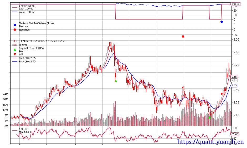
bt交易历史转vectorbt交易信号
bt_entries_mask = bt_transactions[bt_transactions.amount > 0]bt_entries_mask.index = bt_entries_mask.indexbt_exits_mask = bt_transactions[bt_transactions.amount < 0]bt_exits_mask.index = bt_exits_mask.index
bt_entries = pd.Series.vbt.signals.empty_like(ohlcv['Close'])bt_entries.loc[bt_entries_mask.index] = Truebt_exits = pd.Series.vbt.signals.empty_like(ohlcv['Close'])bt_exits.loc[bt_exits_mask.index] = Truevectorbt的回测,可视化
vbt.settings.portfolio['fees'] = 0.075 / 100 #0.0025 # in %bt_pf = vbt.Portfolio.from_signals(ohlcv['Close'], bt_entries, bt_exits, price=ohlcv['Close'].vbt.fshift(1))
bt_pf.trades.plot().show_svg()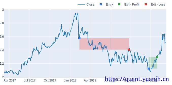
bt和vectorbt手续费对比
bt_commissions = pd.Series(result[0].commissions, index=bt_transactions.index)
vbt_commissions = bt_pf.orders.records_readable.Feesvbt_commissions.index = bt_pf.orders.records_readable.Timestamp
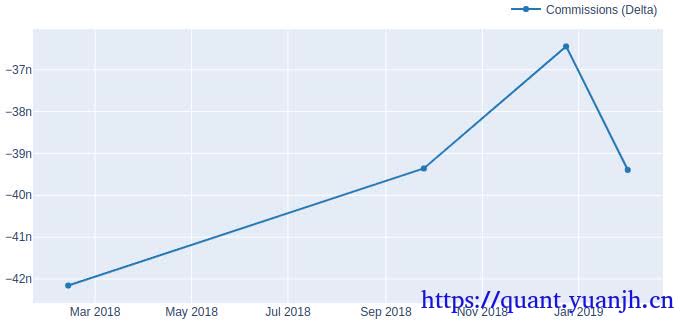
commissions_delta = bt_commissions - vbt_commissionsprint(commissions_delta.head())
2018-02-12 00:00:00+00:00 -4.215589e-082018-09-25 00:00:00+00:00 -3.935966e-082018-12-24 00:00:00+00:00 -3.644546e-082019-02-01 00:00:00+00:00 -3.939400e-08dtype: float64
commissions_delta.rename('Commissions (Delta)').vbt.plot().show_svg()可见,差异约等于0
bt回测报表vectorbt回测报表比对
print('Final Portfolio Value: %.5f' % final_value)print('Profit %.3f%%' % ((final_value - initial_value) / initial_value * 100))print_trade_analysis(result[0].analyzers.ta.get_analysis())print(bt_pf.stats())
Final Portfolio Value: 100.61832Profit 0.618%Trade Analysis Results: Total Open Total Closed Total Won Total Lost 0 2 1 1 Strike Rate Win Streak Losing Streak PnL Net 1 1 1 0.62Start 2017-03-06 00:00:00+00:00End 2019-03-11 00:00:00+00:00Period 0 days 08:12:00Start Value 100.0End Value 100.618319 #和bt基本相等Total Return [%] 0.618319Benchmark Return [%] 21.449275Max Gross Exposure [%] 100.0Total Fees Paid 0.290305Max Drawdown [%] 20.985401Max Drawdown Duration 0 days 04:12:00Total Trades 2 #交易2次,和bt相等Total Closed Trades 2Total Open Trades 0Open Trade PnL 0.0Win Rate [%] 50.0Best Trade [%] 7.934243Worst Trade [%] -6.778074Avg Winning Trade [%] 7.934243Avg Losing Trade [%] -6.778074Avg Winning Trade Duration 0 days 00:27:00Avg Losing Trade Duration 0 days 02:30:00Profit Factor 1.091292Expectancy 0.30916Sharpe Ratio 4.058997Calmar Ratio 3446.385338Omega Ratio 1.024452Sortino Ratio 5.961637Name: Close, dtype: objectvectorbt买卖信号可视化
fig = vbt.make_subplots(specs=[[{"secondary_y": True}]])fig = ohlcv['Close'].vbt.plot(trace_kwargs=dict(name='Price'), fig=fig)
fig = bt_entries.vbt.signals.plot_as_entry_markers(ohlcv['Close'], fig=fig)fig = bt_exits.vbt.signals.plot_as_exit_markers(ohlcv['Close'], fig=fig)
fig.show_svg()
vectorbt策略
指标,信号
# 计算指标RSI = vbt.IndicatorFactory.from_talib('RSI')rsi = RSI.run(ohlcv_wbuf['Open'], timeperiod=[14])
print(rsi.real.shape)(492,)
# 指标转买卖信号vbt_entries = rsi.real_crossed_below(rsi_bottom)vbt_exits = rsi.real_crossed_above(rsi_top)vbt_entries, vbt_exits = pd.DataFrame.vbt.signals.clean(vbt_entries, vbt_exits)
# 买卖信号绘制到价格图中fig = vbt.make_subplots(specs=[[{"secondary_y": True}]])fig = ohlcv['Open'].vbt.plot(trace_kwargs=dict(name='Price'), fig=fig)fig = vbt_entries.vbt.signals.plot_as_entry_markers(ohlcv['Open'], fig=fig)fig = vbt_exits.vbt.signals.plot_as_exit_markers(ohlcv['Open'], fig=fig)
fig.show_svg()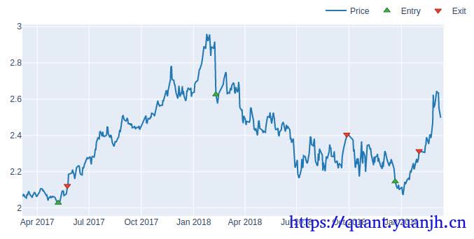
这里需要留意的函数signals.clean
参考官方文档;https://vectorbt.dev/api/signals/accessors/#vectorbt.signals.accessors.SignalsAccessor.clean
SignalsAccessor.clean( *args, entry_first=True, broadcast_kwargs=None, wrap_kwargs=None)Clean signals.
If one array passed, see SignalsAccessor.first(). If two arrays passed, entries and exits, see clean_enex_nb().
SignalsAccessor.first() #下面解释没看懂,但之前代码运行结果为,保留第一个为true的记录,后续置为falsefirst method¶SignalsAccessor.first( wrap_kwargs=None, **kwargs)Select signals that satisfy the condition pos_rank == 0.
clean_enex_nb function¶ #clean_enex_1d_nb()的二维版本,顾名思义应该是多组买卖信号,买在卖前,可能还兼顾将连续的true或false改为单次触发信号clean_enex_nb( entries, exits, entry_first)2-dim version of clean_enex_1d_nb().
clean_enex_1d_nb(). #从信号中取得第一个买卖信号,其中买在卖前,假如2个信号完全相同,则为Noneclean_enex_1d_nb function¶clean_enex_1d_nb( entries, exits, entry_first)Clean entry and exit arrays by picking the first signal out of each.Entry signal must be picked first. If both signals are present, selects none.信号回测结果和差异分析
vbt_pf = vbt.Portfolio.from_signals(ohlcv['Close'], vbt_entries, vbt_exits, price=ohlcv['Close'].vbt.fshift(1))print('Final Portfolio Value (Vectorbt): %.5f' % vbt_pf.final_value())print('Final Portfolio Value (Backtrader): %.5f' % final_value)
Final Portfolio Value (Vectorbt): 98.55972Final Portfolio Value (Backtrader): 100.61832显然,二者回测结果并不匹配
比对交易信号差异
(vbt_entries ^ bt_entries).rename('Entries (Delta)').vbt.signals.plot().show_svg()(vbt_exits ^ bt_exits).rename('Exits (Delta)').vbt.signals.plot().show_svg()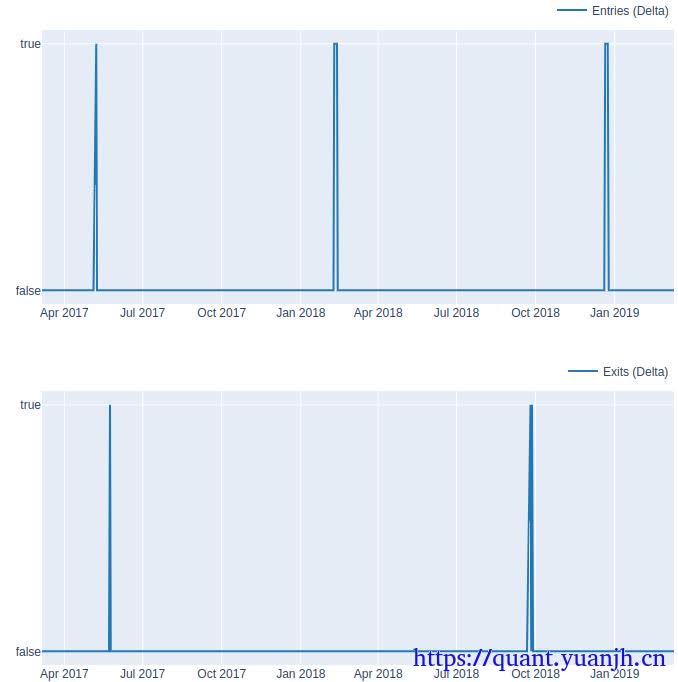
那么差异区间rsi取值是怎样的呢?
# create a selection mask for showing values which are differentmask = vbt_exits ^ bt_exitsprint(vbt_exits[mask]) # show the different ones in vbt_exitsprint(bt_exits[mask]) # show the different ones in bt_exitsprint(rsi.real[mask]) # show the RSI value这几天(mask),vbt_exits和bt_exits信号有差异,所以分别打印vbt_exits和bt_exits在这3天的取值,以及指标原始取值
date2017-05-24 00:00:00+00:00 True2018-09-25 00:00:00+00:00 False2018-09-27 00:00:00+00:00 TrueName: (14, Open), dtype: booldate2017-05-24 00:00:00+00:00 False2018-09-25 00:00:00+00:00 True2018-09-27 00:00:00+00:00 FalseName: Close, dtype: booldate2017-05-24 00:00:00+00:00 66.4482552018-09-25 00:00:00+00:00 63.7828842018-09-27 00:00:00+00:00 66.771968Name: (14, Open), dtype: float64考虑到阈值设置的为65。所以第一组数据是合理的,也就是vbt_exits计算结果是对的。(此时,还有另一个考虑,就是信号发出后,何时触发交易下单,当日还是次日,如果当日,可能存在未来信息隐患)。
bt的指标计算方法用户vectorbt
# backtrader计算的rsi指标rsi_bt_df = pd.DataFrame({ 'rsi': result[0].rsi.get(size=len(result[0])) }, index=[result[0].datas[0].num2date(x) for x in result[0].data.datetime.get(size=len(result[0]))])rsi_bt_df.index = rsi_bt_df.index.tz_localize(tz='UTC')rsi_bt_df.rsi = rsi_bt_df.rsi.shift(1)
# vectorbt计算的rsi指标rsi_vbt_df = pd.DataFrame({ 'rsi': rsi.real.values}, index=rsi.real.index)rsi_vbt_df_mask = (rsi_vbt_df.index >= start_date) & (rsi_vbt_df.index <= end_date) # mask without bufferrsi_vbt_df = rsi_vbt_df.loc[rsi_vbt_df_mask, :]
print(rsi_bt_df.shape)print(rsi_vbt_df.shape)#rsi_bt_df.head(20)#rsi_vbt_df.head(20)(492, 1)(492, 1)计算指标差异和可视化
rsi_delta = rsi_bt_df - rsi_vbt_df#rsi_delta.head(20)rsi_delta.rsi.rename('RSI (Delta)').vbt.plot().show_svg()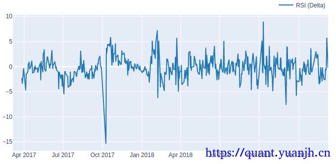
指标同列比对
# Overlappedpd.DataFrame({'RSI (VBT)': rsi_vbt_df['rsi'], 'RSI (BT)': rsi_bt_df['rsi']}).vbt.plot().show_svg()# RSI signal from Backtraderrsi_bt_df.rsi.rename('RSI (BT)').vbt.plot().show_svg()# RSI signal from Vectorbtrsi_vbt_df.rsi.rename('RSI (VBT)').vbt.plot().show_svg()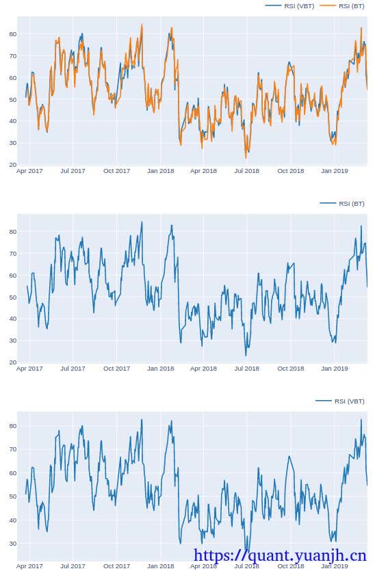
可见,没有明显差异
那么,如果我们可以获得完全相同的结果么?比如使用bt计算的指标,提供给vectorbt做回测。
# 使用bt的指标计算信号vbt_bt_entries = rsi_bt_df.rsi < rsi_bottomvbt_bt_exits = rsi_bt_df.rsi > rsi_topvbt_bt_entries, vbt_bt_exits = pd.DataFrame.vbt.signals.clean(vbt_bt_entries, vbt_bt_exits)
# 信号的可视化fig = vbt.make_subplots(specs=[[{"secondary_y": True}]])fig = ohlcv['Open'].vbt.plot(trace_kwargs=dict(name='Price'), fig=fig)fig = vbt_bt_entries.vbt.signals.plot_as_entry_markers(ohlcv['Open'], fig=fig)fig = vbt_bt_exits.vbt.signals.plot_as_exit_markers(ohlcv['Open'], fig=fig)
fig.show_svg()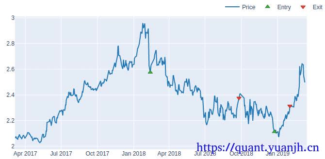
再次绘制信号差异图
(vbt_bt_entries ^ bt_entries).rename('Entries (Delta)').vbt.signals.plot().show_svg()(vbt_bt_exits ^ bt_exits).rename('Exits (Delta)').vbt.signals.plot().show_svg()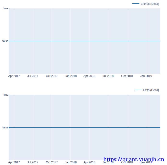
惊不惊喜,意不意外?完全相同,说明之前bt策略和基于vectorbt的策略差异在指标的计算上面。如果指标计算相同,那么二者回测结果也等同。等价于从侧面验证了vectorbt的正确性,毕竟backtrader作为广泛使用的经典框架,出错概率相对低些。
由于上面已经相同,下面信息可以忽略。
# 差异部分的print# create a selection mask for showing values which are differentmask = vbt_bt_exits ^ bt_exitsprint(vbt_bt_exits[mask]) # show the different ones in vbt_bt_exitsprint(bt_exits[mask]) # show the different ones in bt_exitsprint(rsi_bt_df.rsi[mask]) # show the RSI value
# 买卖信号可视化fig = vbt_bt_entries.vbt.signals.plot(trace_kwargs=dict(name='Entries'))vbt_bt_exits.vbt.signals.plot(trace_kwargs=dict(name='Exits'), fig=fig).show_svg()
# vectorbt和backtrader回测方法的终值差异vbt_bt_pf = vbt.Portfolio.from_signals(ohlcv['Close'], vbt_bt_entries, vbt_bt_exits, price=ohlcv['Close'].vbt.fshift(1))print('Final Portfolio Value (Vectorbt): %.5f' % vbt_bt_pf.final_value())print('Final Portfolio Value (Backtrader): %.5f' % final_value)
# vectorbt的交易可视化#print(vbt_bt_pf.trades.records)vbt_bt_pf.trades.plot().show_svg()结论
单纯的持有型策略
hold_pf = vbt.Portfolio.from_holding(ohlcv['Close'])
# 绘制收益图fig = vbt_pf.value().vbt.plot(trace_kwargs=dict(name='Value (pure vectorbt)'))fig = vbt_bt_pf.value().vbt.plot(trace_kwargs=dict(name='Value (vectorbt w/ BT Ind.)'), fig=fig)fig = bt_pf.value().vbt.plot(trace_kwargs=dict(name='Value (Backtrader)'), fig=fig)hold_pf.value().vbt.plot(trace_kwargs=dict(name='Value (Hold)'), fig=fig).show_svg()原文结论:
我们可以看到,vectorbt+backtrader RSI信号生成的投资组合与我们纯backtrader策略生成的投资组完全重叠。然而,正如我们所发现的,纯向量投资组合略有偏离。
这应该提醒你,信号算法实现方式的微小差异,甚至可能在你的策略中产生不同的进入和退出事件!
debug工具箱
vectorbt的交易明细
vbt_pf.orders.records_readable
Order Id Column Timestamp Size Price Fees Side0 0 0 2017-05-08 00:00:00+00:00 49.127363 2.034 0.074944 Buy1 1 0 2017-05-24 00:00:00+00:00 49.127363 2.124 0.078260 Sell2 2 0 2018-02-09 00:00:00+00:00 38.389873 2.714 0.078143 Buy3 3 0 2018-09-27 00:00:00+00:00 38.389873 2.413 0.069476 Sell4 4 0 2018-12-21 00:00:00+00:00 42.921539 2.155 0.069372 Buy5 5 0 2019-02-01 00:00:00+00:00 42.921539 2.298 0.073975 Sellbacktrader的交易明细
bt_pf.orders.records_readable
Order Id Column Timestamp Size Price Fees Side0 0 Close 2018-02-12 00:00:00+00:00 38.760689 2.578 0.074944 Buy1 1 Close 2018-09-25 00:00:00+00:00 38.760689 2.407 0.069973 Sell2 2 Close 2018-12-24 00:00:00+00:00 43.818033 2.126 0.069868 Buy3 3 Close 2019-02-01 00:00:00+00:00 43.818033 2.298 0.075520 Sellbacktrader.vectorbt特定区间总资产
bt_pf.value().iloc[150:].head(20)date2017-10-16 00:00:00+00:00 100.02017-10-17 00:00:00+00:00 100.0,,,2017-11-08 00:00:00+00:00 100.02017-11-09 00:00:00+00:00 100.02017-11-10 00:00:00+00:00 100.0Name: Close, dtype: float64
vbt_pf.value().iloc[150:].head(20)date2017-10-16 00:00:00+00:00 104.2682592017-10-17 00:00:00+00:00 104.2682592017-10-18 00:00:00+00:00 104.268259,,,2017-11-09 00:00:00+00:00 104.2682592017-11-10 00:00:00+00:00 104.268259dtype: float64部分信息可能已经过时