vectorbt学习_03BitcoinDMAC

对应https://vectorbt.dev/getting-started/resources/的第一篇文章
Performance analysis of Moving Average Crossover,比特币，双均线，参数探测和可视化
需要对python工具包，pandas的series和dataframe有大致了解，否则代码的阅读会比较吃力。

文章概述#

一共四部分
第一部分：数据查询和可视化
第二部分：Single window combination，单窗口组合
第三部分：Multiple window combinations，多参数组合测试
第四部分：Strategy comparison，策略比较

第一部分：数据查询和可视化#

主要用来验证，数据查询没问题，需要关注复权情况，避免数据没做复权处理，避免分红，配股引入的回测偏差。

1
数据查询：
2
    ohlcv_wbuf=dbtools.MySQLData.download('510050.XSHG').get() # 自带工具类查询
3

4
数据筛选和过滤
5
    # Create a copy of data without time buffer
6
    wobuf_mask = (ohlcv_wbuf.index >= start_date) & (ohlcv_wbuf.index <= end_date) # mask without buffer 计算指标时需要冗余数据
7
    ohlcv = ohlcv_wbuf.loc[wobuf_mask, :]
8

9
绘制蜡烛图：ohlcv.vbt.ohlcv.plot().show_svg()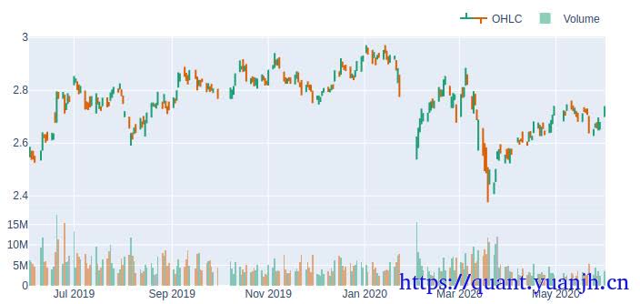

del01

第二部分：Single window combination，单窗口组合#

观察指标的计算和信号的计算，触发等是否符合自己的设计思路，以及那些行情表现好，那些表现差，表现差的能否屏蔽或识别，过滤掉。

1
确保无任何空值：
2
    # there should be no nans after removing time buffer
3
    assert (~fast_ma.ma.isnull().any())
4

5
单次金叉：fast_ma.ma_crossed_above(slow_ma)
6

7
绘制行情，指标，交易信号图：
8
    fig = ohlcv['Open'].vbt.plot(trace_kwargs=dict(name='Price'))
9
    fig = fast_ma.ma.vbt.plot(trace_kwargs=dict(name='Fast MA'), fig=fig)
10
    fig = slow_ma.ma.vbt.plot(trace_kwargs=dict(name='Slow MA'), fig=fig)
11
    fig = dmac_entries.vbt.signals.plot_as_entry_markers(ohlcv['Open'], fig=fig)
12
    fig = dmac_exits.vbt.signals.plot_as_exit_markers(ohlcv['Open'], fig=fig)
13
    fig.show_svg()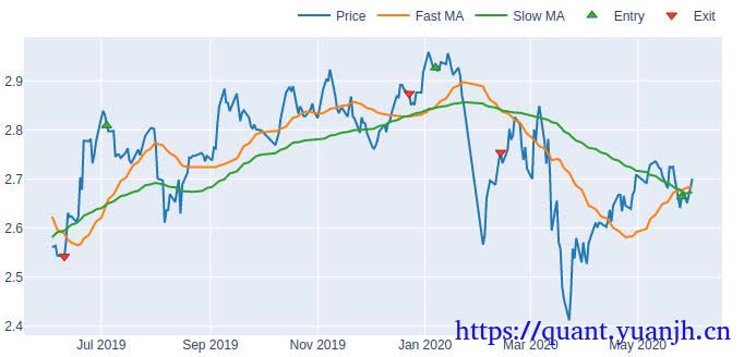

del01

1
信号评估：dmac_entries.vbt.signals.stats(settings=dict(other=dmac_exits))
2

3
Start                       2019-06-03 00:00:00+00:00
4
End                         2020-06-01 00:00:00+00:00
5
Period                                            243 #开始-结束 交易日个数
6
Total                                               3 #交易次数（完整买卖，最后没卖出信号，自动卖出）
7
Rate [%]                                     1.234568 #todo
8
Total Overlapping                                   0 #重叠率，有重叠大概率说明买卖信号组合存在问题
9
Overlapping Rate [%]                              0.0
10
First Index                 2019-07-04 00:00:00+00:00 #推算应该是首次交易日
11
Last Index                  2020-05-26 00:00:00+00:00
12
Norm Avg Index [-1, 1]                       0.123967 #todo
13
Distance -> Other: Min                           21.0 #最小持仓区间，下图A标记距离
14
Distance -> Other: Max                          116.0 #最大持仓区间
15
Distance -> Other: Mean                          68.5 #平均持仓区间
16
Distance -> Other: Std                      67.175144
17
Total Partitions                                    3 #todo
18
Partition Rate [%]                              100.0 #todo
19
Partition Length: Min                             1.0
20
Partition Length: Max                             1.0
21
Partition Length: Mean                            1.0
22
Partition Length: Std                             0.0
23
Partition Distance: Min                          90.0 #2次买入信号最小间距，下图B标记距离
24
Partition Distance: Max                         126.0 #2次买入信号最大间距
25
Partition Distance: Mean                        108.0
26
Partition Distance: Std                     25.455844
27
dtype: object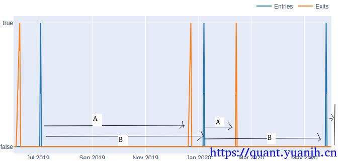

del01

1
买卖信号图：（上图所示）
2
    # Plot signals
3
    fig = dmac_entries.vbt.signals.plot(trace_kwargs=dict(name='Entries'))
4
    dmac_exits.vbt.signals.plot(trace_kwargs=dict(name='Exits'), fig=fig).show_svg()
5

6
交易结果分析：
7
    # Build partfolio, which internally calculates the equity curve
8

9
    # Volume is set to np.inf by default to buy/sell everything
10
    # You don't have to pass freq here because our data is already perfectly time-indexed
11
    dmac_pf = vbt.Portfolio.from_signals(ohlcv['Close'], dmac_entries, dmac_exits)
12

13
    # Print stats
14
    print(dmac_pf.stats())
15
Start                         2019-06-03 00:00:00+00:00
16
End                           2020-06-01 00:00:00+00:00
17
Period                                              243
18
Start Value                                     10000.0 #期初资金
19
End Value                                   9489.187544 #期末资金
20
Total Return [%]                              -5.108125 #总收益率
21
Benchmark Return [%]                           6.669267 #基准回报率
22
Max Gross Exposure [%]                            100.0 #最大总风险，todo
23
Total Fees Paid                              121.927248 #总费用
24
Max Drawdown [%]                              14.772497 #最大回撤
25
Max Drawdown Duration                             138.0 #回撤持续区间
26
Total Trades                                          3 #总交易
27
Total Closed Trades                                   2 #todo
28
Total Open Trades                                     1 #todo
29
Open Trade PnL                               168.683037 #todo
30
Win Rate [%]                                       50.0 #胜率
31
Best Trade [%]                                  0.77486 #0.77%收益率
32
Worst Trade [%]                               -7.528611 #-7.5%收益率
33
Avg Winning Trade [%]                           0.77486 #盈利交易平均收益
34
Avg Losing Trade [%]                          -7.528611 #亏损交易平均收益
35
Avg Winning Trade Duration                        116.0 #盈利交易持有平均周期
36
Avg Losing Trade Duration                          21.0 #亏损交易持有平均周期
37
Profit Factor                                  0.102133 #todo
38
Expectancy                                  -339.747747 #todo
39
dtype: object
40

41
交易历史明细单和可视化
42
    # Plot trades
43
    print(dmac_pf.trades.records)
44
    dmac_pf.trades.plot().show_svg()
45

46
id  col         size  entry_idx  entry_price  entry_fees  exit_idx  exit_price  exit_fees         pnl    return  direction  status  parent_id
47
0   0    0  3553.638170         22     2.807000   24.937656       138    2.842875  25.256373   77.292741  0.007749          0       1          0
48
1   1    0  3418.716194        148     2.940332   25.130406       169    2.733150  23.359660 -756.788234 -0.075286          0       1          1
49
2   2    0  3469.538407        238     2.679682   23.243153       242    2.735000   0.000000  168.683037  0.018143          0       0          2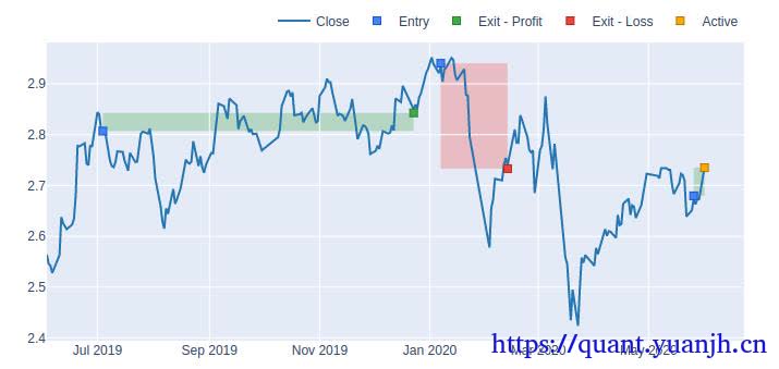

del01

1
多组绩效同列比对
2
    # Equity
3
    fig = dmac_pf.value().vbt.plot(trace_kwargs=dict(name='Value (DMAC)'))
4
    hold_pf.value().vbt.plot(trace_kwargs=dict(name='Value (Hold)'), fig=fig).show_svg()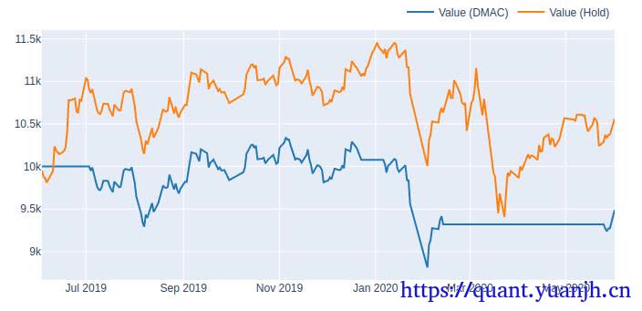

del01

1
可视化动态dashboard调参:
2
    windows_slider.observe(on_value_change, names='value')
3
    on_value_change({'new': windows_slider.value})
4

5
    dashboard = widgets.VBox([
6
        widgets.HBox([widgets.Label('Fast and slow window:'), windows_slider]),
7
        dmac_img,
8
        metrics_html
9
    ])
10
    dashboard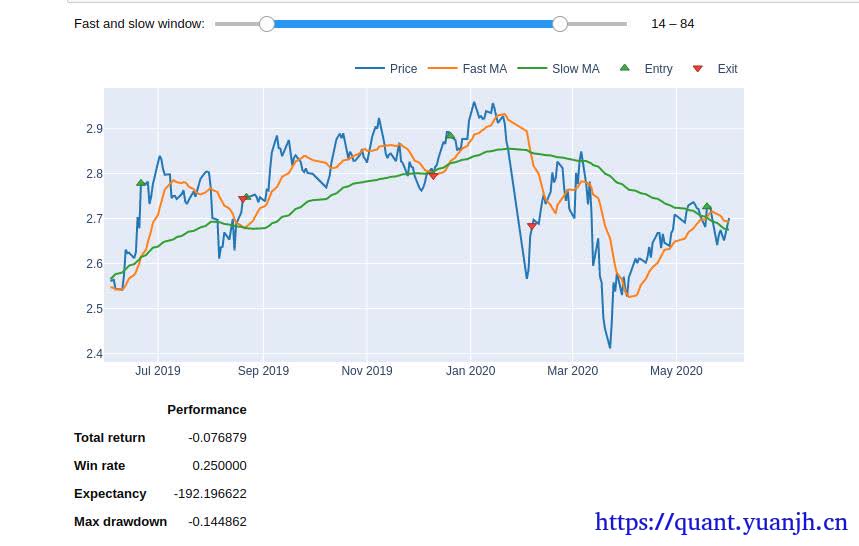

del01

第三部分：Multiple window combinations，多参数组合测试#

对策略涉及的参数进行提取，并测试这些参数组合，获得最佳的参数组合。

1
组合测试：
2
    # Pre-calculate running windows on data with time buffer
3
    fast_ma, slow_ma = vbt.MA.run_combs(
4
        ohlcv_wbuf['Open'], np.arange(min_window, max_window+1),
5
        r=2, short_names=['fast_ma', 'slow_ma'])
6
    print(fast_ma.ma.shape)
7
    print(slow_ma.ma.shape)
8
    print(fast_ma.ma.columns)
9
    print(slow_ma.ma.columns)
10
    (978, 4851)
11
    (978, 4851)
12
    Int64Index([ 2,  2,  2,  2,  2,  2,  2,  2,  2,  2,
13
                ...
14
                96, 96, 96, 96, 97, 97, 97, 98, 98, 99], dtype='int64', name='fast_ma_window', length=4851)
15
    Int64Index([  3,   4,   5,   6,   7,   8,   9,  10,  11,  12,
16
                ...
17
                 97,  98,  99, 100,  98,  99, 100,  99, 100, 100], dtype='int64', name='slow_ma_window', length=4851)
18
    这里需要注意的是4851怎么来的？
19
    2:3->100(98)
20
    3:4->100(97)
21
    98:99->10(2)
22
    99:100->100(1)
23
    组合个数：(98+1)*98/2=4851
24
    可以发现：原始的fast_ma.ma只有一个维度，长度978的float序列，现在多出一个维度,目前的ma多出的维度
25
    fast_ma.ma.columns
26
    Int64Index([ 2,  2,  2,  2,  2,  2,  2,  2,  2,  2,
27
            ...
28
            96, 96, 96, 96, 97, 97, 97, 98, 98, 99], dtype='int64', name='fast_ma_window', length=4851)
29

30
组合测试的信号生成：
31
    表面和单指标相同
32
    dmac_entries = fast_ma.ma_crossed_above(slow_ma)
33
    print(dmac_entries.columns) # the same for dmac_exits
34
    MultiIndex([( 2,   3),
35
            ( 2,   4),
36
            ( 2,   5),
37
            ( 2,   6),
38
            ( 2,   7),
39
            ( 2,   8),
40
            ( 2,   9),
41
            ( 2,  10),
42
            ( 2,  11),
43
            ( 2,  12),
44
            ...
45
            (96,  97),
46
            (96,  98),
47
            (96,  99),
48
            (96, 100),
49
            (97,  98),
50
            (97,  99),
51
            (97, 100),
52
            (98,  99),
53
            (98, 100),
54
            (99, 100)],
55
           names=['fast_ma_window', 'slow_ma_window'], length=4851)
56
     这里需要注意的fast_ma和slow_ma的columns本都是单个int取值，crossed后自动，由于columns不同组合，自动生成multiindex了。
57
组合测试回测评估
58
    # Build portfolio
59
    dmac_pf = vbt.Portfolio.from_signals(ohlcv['Close'], dmac_entries, dmac_exits)
60
    dmac_perf = dmac_pf.deep_getattr(metric) #metric = 'total_return'
61

62
    print(dmac_perf.shape)
63
    print(dmac_perf.index)
64
    (4851,)
65
MultiIndex([( 2,   3),
66
            ( 2,   4),
67
            ( 2,   5),
68
            ( 2,   6),
69
            ( 2,   7),
70
            ( 2,   8),
71
            ( 2,   9),
72
            ( 2,  10),
73
            ( 2,  11),
74
            ( 2,  12),
75
            ...
76
            (96,  97),
77
            (96,  98),
78
            (96,  99),
79
            (96, 100),
80
            (97,  98),
81
            (97,  99),
82
            (97, 100),
83
            (98,  99),
84
            (98, 100),
85
            (99, 100)],
86
           names=['fast_ma_window', 'slow_ma_window'], length=4851)
87
      可见：dmac_perf其实完成column转index，同时猜测如果metric含有多个取值，那么dmac_perf.columns也会增加。
88

89
最佳参数组：
90
    # Calculate performance of each window combination
91
    dmac_perf = dmac_pf.deep_getattr(metric) #metric = 'total_return'
92
    dmac_perf.idxmax()
93
2维参数热力图可视化：
94
    # Convert this array into a matrix of shape (99, 99): 99 fast windows x 99 slow windows
95
    dmac_perf_matrix = dmac_perf.vbt.unstack_to_df(symmetric=True,
96
        index_levels='fast_ma_window', column_levels='slow_ma_window')
97
    dmac_perf_matrix.vbt.heatmap(
98
        xaxis_title='Slow window',
99
        yaxis_title='Fast window').show_svg()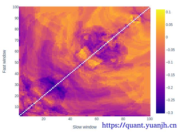

del01

交互式图表，以及gif动图的生成，有点复杂了，感觉用处不大，不深究
del01

第四部分：Strategy comparison，策略比较#

这一部分不是很懂干嘛用的，这个步骤的目标是什么，多个滚动时间窗口平均更能说明策略好坏？
规避起始-结束时间区间，引入的回测误差，将策略运行周期也看做策略参数，比如,fast-slow-range,5-10-40，就是5日10日的双均线策略，在40日为一个单元情况下的收益分布。
但个人感觉类似40日这样可比性不强，由于波动性随着时间大概率有变化的，所以震荡市向单边市场靠近时，必然导致统计数据不准的情况。所以我也不是非常肯定，这种测试是用来说明什么的。
简单来说，这种策略测试，有意义，但意义不大，只能笼统看做是对策略开始看时间的敏感性测试。或是策略对单笔交易鲁棒性体现指标。

1
时间区间回测：
2
    open_roll_wbuf, split_indexes = ohlcv_wbuf['Open'].vbt.range_split(
3
    range_len=(ts_window + time_buffer).days, n=ts_window_n)
4

5
    print(open_roll_wbuf.shape)
6
    print(open_roll_wbuf.columns)
7
    (465, 50)
8
    Int64Index([0, 1, 2, 3, 4, 5, 6, 7, 8, 9, 10, 11, 12, 13, 14, 15, 16, 17, 18, 19, 20, 21, 22, 23, 24, 25, 26, 27, 28, 29, 30, 31, 32, 33, 34, 35, 36, 37, 38, 39, 40, 41, 42, 43, 44, 45, 46, 47, 48, 49], dtype='int64', name='split_idx')
9
    比较容易理解，原始的1列数据，copy出50列，列索引从0-49。
10

11
    # This will calculate moving averages for all date ranges and window combinations
12
    fast_ma_roll, slow_ma_roll = vbt.MA.run_combs(
13
        open_roll_wbuf, np.arange(min_window, max_window+1),
14
        r=2, short_names=['fast_ma', 'slow_ma'])
15

16
    print(fast_ma_roll.ma.shape)
17
    print(fast_ma_roll.ma.columns)
18
    (465, 242550) # 4851*50=242550
19
    MultiIndex([( 2,  0),
20
                ( 2,  1),
21
                ( 2,  2),
22
                ( 2,  3),
23
                ( 2,  4),
24
                ( 2,  5),
25
                ( 2,  6),
26
                ( 2,  7),
27
                ( 2,  8),
28
                ( 2,  9),
29
                ...
30
                (99, 40),
31
                (99, 41),
32
                (99, 42),
33
                (99, 43),
34
                (99, 44),
35
                (99, 45),
36
                (99, 46),
37
                (99, 47),
38
                (99, 48),
39
                (99, 49)],
40
               names=['fast_ma_window', 'split_idx'], length=242550)
41
     从原始的常规columns数字索引，变成数字pair的二维multi索引。
42
    # Generate crossover signals
43
    dmac_entries_roll = fast_ma_roll.ma_crossed_above(slow_ma_roll)
44
    print(dmac_entries_roll.columns)
45
    MultiIndex([( 2,   3,  0),
46
            ( 2,   3,  1),
47
            ( 2,   3,  2),
48
            ( 2,   3,  3),
49
            ( 2,   3,  4),
50
            ( 2,   3,  5),
51
            ( 2,   3,  6),
52
            ( 2,   3,  7),
53
            ( 2,   3,  8),
54
            ( 2,   3,  9),
55
            ...
56
            (99, 100, 40),
57
            (99, 100, 41),
58
            (99, 100, 42),
59
            (99, 100, 43),
60
            (99, 100, 44),
61
            (99, 100, 45),
62
            (99, 100, 46),
63
            (99, 100, 47),
64
            (99, 100, 48),
65
            (99, 100, 49)],
66
           names=['fast_ma_window', 'slow_ma_window', 'split_idx'], length=242550)
67
     信号由原来的2维pair变成3维pair。
68

69
    # Calculate the performance of the DMAC Strategy applied on rolled price
70
    # We need to specify freq here since our dataframes are not more indexed by time
71
    dmac_roll_pf = vbt.Portfolio.from_signals(close_roll, dmac_entries_roll, dmac_exits_roll, freq=freq)
72

73
    dmac_roll_perf = dmac_roll_pf.deep_getattr(metric)
74

75
    print(dmac_roll_perf.shape)
76
    print(dmac_roll_perf.index)
77
    (242550,)
78
    MultiIndex([( 2,   3,  0),
79
                ( 2,   3,  1),
80
                ( 2,   3,  2),
81
                ( 2,   3,  3),
82
                ( 2,   3,  4),
83
                ( 2,   3,  5),
84
                ( 2,   3,  6),
85
                ( 2,   3,  7),
86
                ( 2,   3,  8),
87
                ( 2,   3,  9),
88
                ...
89
                (99, 100, 40),
90
                (99, 100, 41),
91
                (99, 100, 42),
92
                (99, 100, 43),
93
                (99, 100, 44),
94
                (99, 100, 45),
95
                (99, 100, 46),
96
                (99, 100, 47),
97
                (99, 100, 48),
98
                (99, 100, 49)],
99
               names=['fast_ma_window', 'slow_ma_window', 'split_idx'], length=242550)
100
数据格式转换：
101
    # Unstack this array into a cube
102
    dmac_perf_cube = dmac_roll_perf.vbt.unstack_to_array(
103
        levels=('fast_ma_window', 'slow_ma_window', 'split_idx'))
104

105
    print(dmac_perf_cube.shape)
106
    (98, 98, 50)
107
绘制fast-slow windows回测结果图
108
    # For example, get mean performance for each window combination over all date ranges
109
    heatmap_index = dmac_roll_perf.index.levels[0]
110
    heatmap_columns = dmac_roll_perf.index.levels[1]
111
    # np.nanmean取平均,所以最后是二维图而非立方体,https://www.python100.com/html/96013.html
112
    heatmap_df = pd.DataFrame(np.nanmean(dmac_perf_cube, axis=2), index=heatmap_index, columns=heatmap_columns)
113
    heatmap_df = heatmap_df.vbt.make_symmetric()
114

115
    heatmap_df.vbt.heatmap(
116
        xaxis_title='Slow window',
117
        yaxis_title='Fast window',
118
        trace_kwargs=dict(zmid=0, colorscale='RdBu')).show_svg()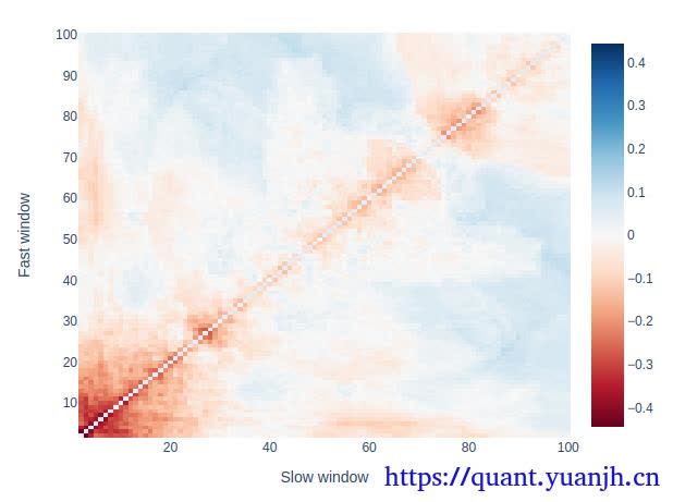

del01

查看特定fast-slow windows参数组合的收益分布

1
# Or for example, compare a pair of window combinations using a histogram
2
window_comb1 = (10, 22)
3
window_comb2 = (73, 77)
4

5
# Get index of each window in strat_cube
6
fast1_idx = np.where(heatmap_df.index == window_comb1[0])[0][0]
7
slow1_idx = np.where(heatmap_df.columns == window_comb1[1])[0][0]
8
fast2_idx = np.where(heatmap_df.index == window_comb2[0])[0][0]
9
slow2_idx = np.where(heatmap_df.columns == window_comb2[1])[0][0]
10

11
print(fast1_idx, slow1_idx, fast2_idx, slow2_idx)
12

13
dmac_comb1_perf = dmac_perf_cube[fast1_idx, slow1_idx, :]
14
dmac_comb2_perf = dmac_perf_cube[fast2_idx, slow2_idx, :]
15

16
pd.DataFrame({str(window_comb1): dmac_comb1_perf, str(window_comb2): dmac_comb2_perf}).vbt.histplot().show_svg()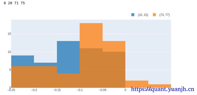

del01
由于每个参数对应50个不同的时间range，所以直方图列取值sum=50，可以近似看做特定参数组合的收益分布情况。

todo：补充，可以绘制各个参数的收益分布情况，可能更明显，选择高均值，低方差的参数组合，只是数据可能较多，100*100个组合。
可以笼统-》细化的思路处理，比如slow：1-》100，分成10个区间，1-》10，10-》20，fast也是类似的，这样可以找出平均收益最大的格子，锁定slow-fast区间，比如slow[10,20],fast:[20-30],之后再二次探测，类似迭代找局部最优解的思路。

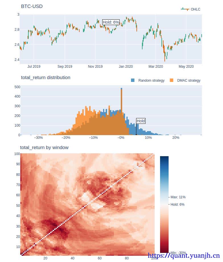
用双均线策略和单纯的持有，以及随机买卖策略回测结果比对

1
pd.DataFrame({
2
    'Random Strategy': rand_roll_perf,
3
    'Hold Strategy': hold_roll_perf,
4
    'DMAC Strategy': dmac_roll_perf,
5
}).vbt.histplot(
6
    xaxis_title=metric,
7
    yaxis_title='Cumulative # of tests',
8
    trace_kwargs=dict(cumulative_enabled=True)).show_svg() # cumulative_enabled累加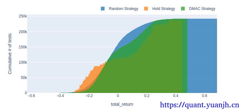

del01

首先纵轴的250k是什么？

1
print(rand_roll_perf.shape)
2
(242550,)
3
就是之前的4851*50=242550

其次累积图，有点让人看不懂，不妨改为非累积

1
pd.DataFrame({
2
    'Random Strategy': rand_roll_perf,
3
    'Hold Strategy': hold_roll_perf,
4
    'DMAC Strategy': dmac_roll_perf,
5
}).vbt.histplot(
6
    xaxis_title=metric,
7
    yaxis_title='Cumulative # of tests',
8
    trace_kwargs=dict(cumulative_enabled=False)).show_svg()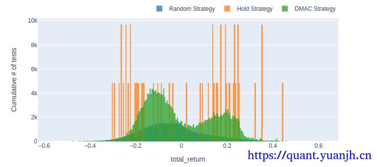

del01
颜色上会有遮挡，hold策略收益分布较极端，dmac绿色部分，random对应绿色内部的深色部分。
这个能体现什么呢？也不是很懂，怎么评估优劣?，目前我也没看太懂。

时间维度绘制三种策略的收益变化图(平均收益)

1
pd.DataFrame({
2
    'Random strategy': rand_roll_perf.groupby('split_idx').mean(),
3
    'Hold strategy': hold_roll_perf.groupby('split_idx').mean(),
4
    'DMAC strategy': dmac_roll_perf.groupby('split_idx').mean()
5
}).vbt.plot(
6
    xaxis_title='Split index',
7
    yaxis_title='Mean %s' % metric).show_svg()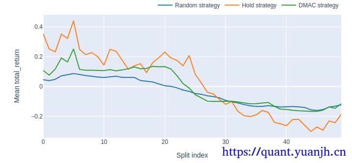

del01
能体现什么信息呢？
大致体现随着时间窗口移动，策略整体有效性（由于上面用的mean平均收益，dmac_roll_perf.groupby(‘split_idx’).mean()，所以可以认为双均线策略的综合有效性）。不过，由于不同参数的策略其实是完全不同的策略，所以感觉这组数据用来评估策略-时间关联性的说服力并不强。

下面是特定参数组合的例子。大致看出各参数组合策略收益稳定性。这个还是有一定说服力的。
del01

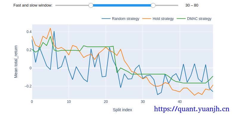
这个重点观察
先选定一组fast-slow windows参数
首先，思考下，本周一启动策略和下周一启动策略，那么策略执行结果相同么？肯定不同，如果本周触发交易信号，则由于交易序列不同，所以形成trads历史不同，最终收益自然也不同（策略对起始时间的敏感性，策略对单笔收益的鲁棒性，是否依靠某一笔收益取得正向结果）。由于我们不能乐观的估计，目前启动策略就一定位于高点上，所以需要采用窗口回测（windows=n）方法，得到一组收益数据。那么这组收益数据，就可以看做，是策略运行一个windows单位的最终收益分布。最优收益，最差收益，平均收益，以及收益稳定性。
所以重点关注这组fast-slow windows参数下:
01，理想的曲线时，都在0轴上方，越向上越好，均值大，波动小
02，是否稳定0轴上方，如果0附近随机波动，说明类似掷筛子，如果有正均值还行，负均值就不理想了。
03，最高，最低点距离，希望波动小，波动大了，很可能今天进去，恰好赶上最差的周期，windows天后，悲提最差收益。
04，收益权限最高点，对应windows时间区间行情长相，说明策略对这一类行情有偏好。想办法筛选出。
同理，收益最低点，对应windows时间区间行情长相，说明策略对这一类行情有排斥。想办法过滤掉。

黄金矿工

文章概述#

第一部分：数据查询和可视化#

第二部分：Single window combination，单窗口组合#

第三部分：Multiple window combinations，多参数组合测试#

第四部分：Strategy comparison，策略比较#